#' Create ridgelines from a digital elevation model (dhm)
#'
#' dhm: path to a dhm that can be imported using terra::rast
#' n_lines: how many lines / polygons do you want to draw? Default is 50
#' vspace: vertical space between lines, in units provided by the dhm. This overrides n_lines
#' fac: How much of the space between the lines should be occupied by the hightest elevation?
#' point_density: Density of the point samples used to extract elevation. Defaults to the inverse of the raster resolution
#' geom_type: What should the output geometry type be? Can be LINESTRING or POLYGON
create_ridges <- function(dhm, n_lines = 50, vspace = NULL, fac = 2, point_density = NULL, geom_type = "LINESTRING"){

  library(sf)
  library(terra)
  library(purrr)

  # extract the extent of the dhm as a vector
  ex <- ext(dhm) %>%
    as.vector()

  # If vspace is NULL (default), then vspace is calculated using n_lines
  if(is.null(vspace)){
    vspace <- (ex["ymax"] - ex["ymin"])/n_lines
  }


  point_density <- if(is.null(point_density)){1/terra::res(dhm)[2]}

  # Defines at what y-coordinates elevation should be extracted
  heights <- seq(ex["ymin"], ex["ymax"], vspace)

  # calculates the x/y coordinates to extract points from the dhm
  mypoints_mat <- map(heights, function(height){
    matrix(c(ex["xmin"], height, ex["xmax"], height), ncol = 2, byrow = TRUE) %>%
      st_linestring()
  }) %>%
    st_as_sfc() %>%
    st_line_sample(density = point_density,type = "regular") %>%
    st_as_sf() %>%
    st_cast("POINT") %>%
    st_coordinates()


  # extracts the elevation from the dhm
  extracted <- terra::extract(dhm, mypoints_mat) %>%
    cbind(mypoints_mat) %>%
    as_tibble()

  # calculates the factor with which to multiply elevation, based on "fac" and the maximum elevation value
  fac <- vspace*fac/max(extracted[,1], na.rm = TRUE)

  # calculates the coordinats of the ridge lines
  coords <-extracted %>%
    filter(!is.na(extracted[,1])) %>%
    split(.$Y) %>%
    imap(function(df, hig){
      hig <- as.numeric(hig)
      Y_new <- hig+pull(df[,1])*fac
      matrix(c(df$X, Y_new), ncol = 2)
    })

  # creates LINESTRING or POLYGON, based on the "geom_type"
  geoms <- if(geom_type == "LINESTRING"){
    map(coords, ~st_linestring(.x))
  } else if(geom_type == "POLYGON"){
    imap(coords, function(x, hig){
      hig <- as.numeric(hig)

      first <- head(x, 1)
      first[,2] <- hig
      last <- tail(x, 1)
      last[,2] <- hig

      st_polygon(list(rbind(first, x, last, first)))
    })
  } else{
    stop(paste0("This geom_type is not implemented:",geom_type,". geom_type must be 'LINESTRING' or 'POLYGON'"))
  }

  # adds the CRS to the output sfc
  dhm_crs <- crs(dhm)

  if(dhm_crs == "") warning("dhm does not seem to have a CRS, therefore the output does not have a CRS assigned either.")

  geoms %>%
    st_sfc() %>%
    st_set_crs(dhm_crs)

}

# A helper function to creteate a polygon from the extent of a (dhm) raster
st_bbox_rast <- function(rast_obj){

  library(terra)
  library(sf)

  ex <- ext(rast_obj) %>%
    as.vector()

  matrix(c(ex[1],ex[3],ex[1], ex[4],ex[2], ex[4],ex[2],ex[3],ex[1],ex[3]),ncol = 2, byrow = TRUE) %>%
  list() %>%
  st_polygon() %>%
    st_sfc(crs = crs(rast_obj))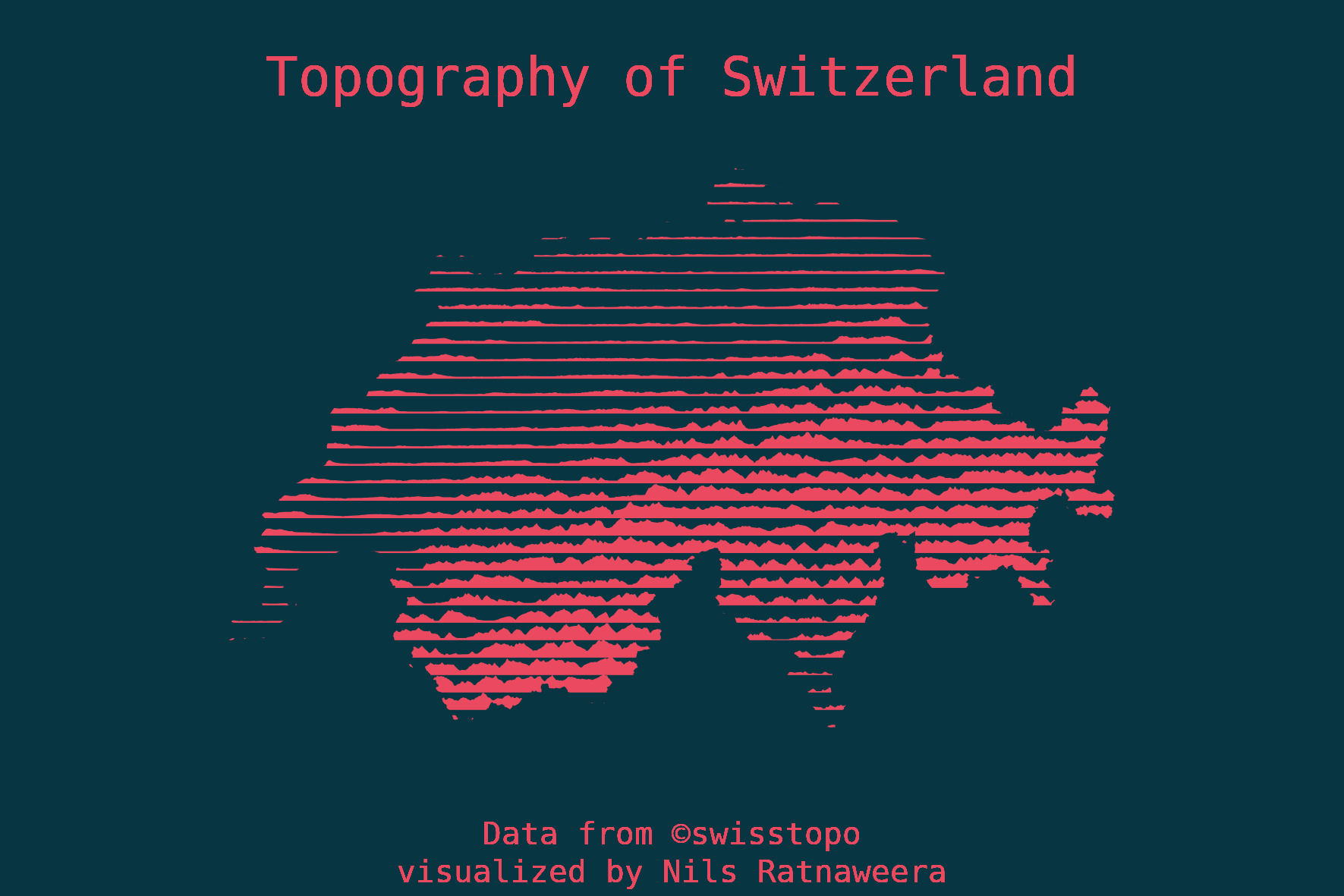
}“So beautiful that it hurts”1 Bauhasaurus wrote in his tweet, posting an image by Carla Martínez Sastre. The artist had used a beautiful, clever and minimalistic way to visualize the topography of South America.
The way I understand it, Carla drew “horizontal” (latitudanal) elevation profiles at equal intervals over the continent and filled these elevation profiles to visualize not only the continent’s topography, but also implicitly showing it’s borders.
I found this a very nice approach and tried recreating this idea with R for my home country, Switzerland. I’m quite happy with the result, however there is still a lot of room for improvement. I’ve packed the approach into generic functions, see below for the complete source code. Check below to see the source code.
Create some generic functions
Import data and use the functions
Code
library(sf)
library(terra)
library(dplyr)
library(purrr)
library(ggplot2)
# library(ragg)


dhm <- terra::rast("data-git-lfs/DHM25/DHM200.asc")
crs(dhm) <- "epsg:21781"


switzerland_21781 <- sf::read_sf("data-git-lfs/swissboundaries/swissBOUNDARIES3D_1_3_TLM_LANDESGEBIET.shp") %>%
  st_union() %>%
  st_transform(21781)

mymask <- st_bbox_rast(dhm) %>%
  st_buffer(5000) %>%
  st_difference(switzerland_21781)


sf_obj <- create_ridges(dhm,n_lines = 35, fac = 1.1,geom_type = "POLYGON")

# bg_color <- "#27363B"
bg_color <- Sys.getenv("plot_bg_col")
fg_color <- "#EB4960"
family <- "FreeMono"


bbox_switz <- st_bbox(switzerland_21781)
bbox_switz_enlarge <- st_buffer(st_as_sfc(bbox_switz),50000)
lims <- st_bbox(bbox_switz_enlarge)
xlims =  lims[c("xmin","xmax")]
ylims = lims[c("ymin","ymax")]

asp <- diff(ylims)/diff(xlims)
Code
myplot <- ggplot(sf_obj) +
  geom_sf(color = "NA", fill = fg_color)  +
  geom_sf(data = mymask, color = "NA", fill = bg_color) +
  # geom_sf(data = bbox_switz_enlarge, fill = "NA") +
  ggtext::geom_richtext(aes(x = median(xlims), y = quantile(ylims,0.95), label = "Topography of Switzerland"), family = family, fill = NA, label.color = NA, hjust = 0.5, size = 6, color = fg_color)+
  ggtext::geom_richtext(aes(x = median(xlims), y = ylims["ymin"], label = "Data from ©swisstopo<br>visualized by Nils Ratnaweera"), family = family, fill = NA, label.color = NA, hjust = 0.5, size = 3.5, color = fg_color)+
  theme_void() +
  theme(plot.background = element_rect(fill = bg_color,color = NA)) +
  coord_sf(datum = 21781,xlim =  xlims, ylim = ylims);
Footnotes
Original (Esp): “Tan linda que duele.”↩︎