How open are our cantons?

Just a couple of years ago, we never used geodata from cantons when doing a Swiss wide project. The data was just too inhomogeneous, too hard to assemble and to expensive to acquire. Now, with geodienste.ch up and running, this task has become much much simpler. Or so I thought.

To be fair, the platform is amazing (although lacking an API) and most cantons are very accommodating, providing the data freely. Some cantons however, are still extremely restrictive with their publicly funded data, asking for close to 50’000 CHF (!!) for commercial use of their data! I’m lucky enough to be working in a research project at a university, but I can’t help but mourn the opportunities this data could be used for if it was provided freely.

Anyway, this experience lead me to the question: Which cantons are most open in their data sharing policy? Which cantons are more restrictive? To answer this question, I scraped the title-page of each of the 23 datasets on geodienste.ch and visualized the results.

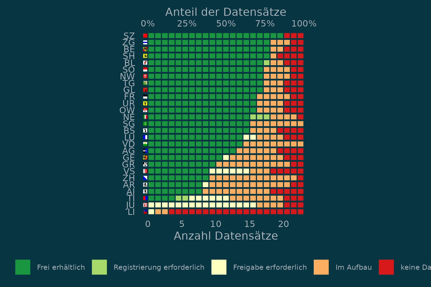
geodienste.ch provides three different methods to obtain the data. Either 1) the data is freely available without registration, 2) the data is freely available after registering on the website or 3) the canton needs to approve your request. This last method can mean that you will be grated approval within a few hours, or that you need to wait a couple of days to receive an email asking you to pay horrendous amounts (if you want to use it commercially).

The results show that most datasets available on the website are offered freely and without the need of registration. Some few datasets require registration, and only 6 cantons feel the need to manually approve and potentially charge certain datasets. Foremost, the cantons Jura, Ticino and Valais heavily guard their data and require approval on a large number of their datasets.

Most cantons offer between 10 and 15 datasets on geodienste.ch. The canton Schwyz has the highest number of datasets online (20), while Zug, Bern and Schaffhausen share second place with 18 datasets each. All provide their data to unregistered users freely. Good for you, that is the way to go!

show code for webscraping

library(httr)
library(xml2)
library(rvest)
library(tidyverse)

services <- read_html("https://geodienste.ch/versions_overview") %>%
  html_elements("a") %>%
  html_attr("href")

services <- services[str_detect(services, "/services/")]


kantone <- read_html("https://geodienste.ch/services/av") %>%
  html_elements(".wappen-kt") %>%
  html_text()

kantone <- str_trim(kantone)
wappen <- read_html("https://geodienste.ch/services/av") %>%
  html_elements(".wappen-kt") %>%
  html_elements("img") %>%
  html_attr("src")

kantone2 <- paste0(kantone,str_extract(wappen, "\\.\\w{3}$"))


map2(kantone2, wappen, function(x,y){
  download.file(paste0("https://geodienste.ch/",y),file.path("wappen",x))
})

fi <- list.files("wappen/",".png", full.names = TRUE)

file.rename(fi, str_remove(fi, " "))


myres <- map(services, function(url_i){
  res <- read_html(paste0("https://geodienste.ch/",url_i)) %>%
    # html_elements(".canton-table") %>%
    html_table() %>%
    magrittr::extract2(1)
  
  res <- res %>% 
    janitor::clean_names()
  
  res %>%
    filter(!is.na(info))
})

res2 <- map2_dfr(myres, services, function(mydf, serv){
  mydf <- mydf[,1:3]
  mydf$services <- serv
  mydf
})

write_csv(res2, "geodienste-raw.csv")

show code for data preparation

library(tidyverse)
library(sf)
library(cowplot)


res2 <- read_csv("geodienste-raw.csv")
facs <- c("Frei erhältlich","Registrierung erforderlich","Freigabe erforderlich","Im Aufbau", "keine Daten")

res3 <- res2 %>%
  separate(verfugbarkeit, c("verfugbarkeit","verfugbarkeit2"), sep = "\\n\\s+") %>% 
  select(-verfugbarkeit2) %>%# verfugbarkeit2 seems to be erroneous 
  mutate(
    erhaeltlich_ab = str_extract(verfugbarkeit, "\\d{2}\\.\\d{2}\\.\\d{4}"),
    verfugbarkeit = str_remove(verfugbarkeit, "\\s\\(.+\\)")
  ) %>%
  rename(kanton = x)


res3_wide <-res3 %>%
  group_by(kanton, verfugbarkeit) %>%  
  count() %>%
  mutate(verfugbarkeit_code = paste0("verf",as.integer(factor(verfugbarkeit, facs)))) %>%
  ungroup() %>%
  select(-verfugbarkeit) %>%
  pivot_wider(names_from = verfugbarkeit_code, values_from = n,values_fill = 0) %>%
  select(kanton, order(colnames(.))) %>%
  arrange(across(starts_with("verf")))


res4 <- res3 %>%
  mutate(
    kanton = factor(kanton, levels = res3_wide$kanton, ordered = TRUE),
    verfugbarkeit = factor(verfugbarkeit, levels = facs, ordered = TRUE),
    x = 1
  ) 


wappen_df <- tibble(file = list.files("wappen",full.names = TRUE)) %>%
  mutate(
    kanton = str_extract(file, "[A-Z][A-Z]"),
) %>%
  left_join(res3_wide, ., by = "kanton") %>%
  mutate(y = row_number())

show code for creating the plot

cols <- rev(RColorBrewer::brewer.pal(5, "RdYlGn"))

plot_bg_col <- Sys.getenv("plot_bg_col") 
text_col <- Sys.getenv("text_col")

p <- res4 %>%
  ggplot(aes(x, kanton, fill = verfugbarkeit)) + 
  geom_col(position = position_stack(reverse = TRUE), color = plot_bg_col) +
  pmap(select(wappen_df, file, y), function(file, y){draw_image(file, x = -0, y = y, width = 0.8, height = 0.6,hjust = 1,vjust = 0.5)}) +
  scale_fill_manual("Status",values = cols) +
  scale_x_continuous("Anzahl Datensätze",sec.axis = sec_axis(~./23,"Anteil der Datensätze", labels = scales::percent_format())) +
  # guides(fill = guide_legend(title.position = "top",title.hjust = 0.5)) +
  theme_minimal() +
  theme(legend.position = "bottom",
        axis.title.y = element_blank(), 
        panel.grid = element_blank(),
        plot.background = element_rect(fill = plot_bg_col, colour = NA),
        panel.background = element_rect(fill = plot_bg_col, colour = NA),
        legend.text = element_text(size = 7),
        legend.title = element_blank(),
        text = element_text(colour = text_col),
        axis.text = element_text(colour = text_col)
        ) +
  coord_equal() #+ theme(plot.background = element_rect(fill = "plot_bg_col"))

ggsave("preview.png", width = 15, height = 10, units = "cm",scale = 1.4)